This is where we will post the homework for the class.

Homework 1 (Due 1/17):

All the problems are out of the textbook. When the textbook talks about a computer program, like DiffEq, you should just use the program on our website instead.

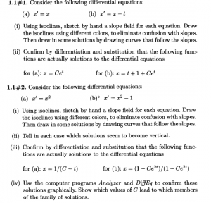
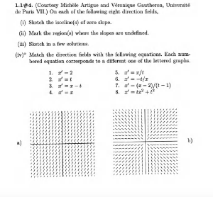
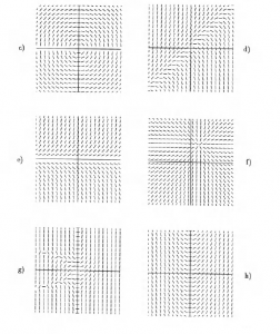
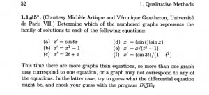
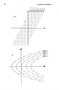
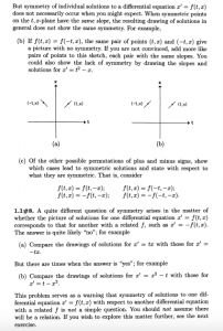
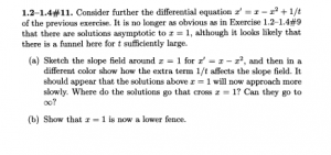
Also, because some copies of the textbook have not arrived, I am including screen shots of the relevant problems from Hubbard and West:

1.1: #1

1.1: #2 (i – iv) [For (iv), you can just mark a few values of C on a plot that sketches solutions, made either by hand or by computer.]

1.1: #4

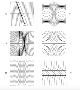
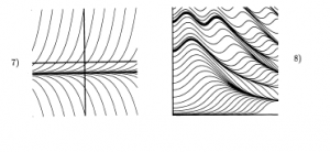
1.1: #5

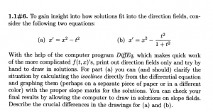
1.1: #6

1.2 – 1.4: #1

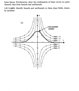
1.2 – 1.4: #2

1.2 – 1.4: #7

1.2 – 1.4: #9

1.2 – 1.4: #10

Homework 2 (due FRIDAY 1/26):

1.1: #7 a, b
1.1: #8
1.2 – 1.4: #11 (a – d)
1.2 – 1.4: #15
2.1: 1 (a-c)
2.1: 2 (a – c)
2.2-2.3: 4 (a, g)

Homework 3 (due FRIDAY 2/2):

2.2-2.3: #3 (You don’t have to hand anything in about the computer drawings; just take a few moments to compare your results with what the tool on our website gives.)
2.2-2.3: #6
2.2-2.3: #7
2.2-2.3: #8
2.2-2.3: #9
2.2-2.3: #10 (a,b,d) (You don’t have to hand in anything involving the computer part, but you should convince yourself that the solutions that you get match what the computer draws.)
2.6: #1 (a, c, f)
2.7: #1

Homework 4 (short due to the midterm; due WEDNESDAY Feb. 14)

3.1-3.2: #2 (by the “Euler approximation solution” they just mean the solution you get by connecting the points (t_n,x_n) with straight lines)
3.1-3.2: #5
3.1-3.2: #6
4.1-4.2: #1

Homework 5 (due Friday Feb. 23)

It is written out here: Math 106 Homework #5

Homework 6 (due Friday Mar. 2)

7.3 #3, #4 (a),
7.4 #1 (a, b), #3 (a-c)
7.5 #2, #4 (a)
7.7 #1

Homework 7 (due Friday Mar. 9)

7.7: #6, #10
8.1: #1.(i), #5 (for b, you should just use the computer program to compare the actual equation with its linearization, and write a little bit about where this approximation is accurate)
7.5: #6 (b, c; see the elaboration on this below), #7

Extra Credit: 7.5: #8

A remark about language for 7.5: #6 —

This question just means that you are to consider the system x’=Ax, where A is a 2-by-2 matrix, and x is a vector with two components. The “phase plane” refers to the plane in which you would plot the vector x, while the word trajectory just means a solution of this system. So, for the first part of part (b) of the question, for example, you are supposed to show that the plot of a solution with initial condition on the eigenvector with positive eigenvalue stays along that eigenvector and moves away from the origin.